Optical time-domain reflectometry (OTDR)
Measuring loss along an optical fiber from one end by sending short light pulses into it and timing the Rayleigh backscatter and reflections that return, at 102 m of fiber per microsecond of round trip. One trace shows the fiber's attenuation, the loss and position of each splice and connector, and the location of a break.
Optical time-domain reflectometry (OTDR) maps a fiber from one end: an optical time-domain reflectometer sends short light pulses into the fiber and times the light that comes back, both the Rayleigh backscatter produced continuously along the glass and the Fresnel reflections from connectors, breaks and the far end. The round-trip delay gives the distance, , which is 102 m of fiber per microsecond for a group index , and the level of the backscatter at each distance gives the loss accumulated up to that point. One trace therefore shows the attenuation of the fiber, the loss and position of every splice and connector, and the location of a break or of the far end.
The instrument combines a pulsed laser diode, a coupler or circulator that sends each pulse into the fiber and routes the returning light to the receiver, usually an avalanche photodiode, and a digitizer that samples the return. The backscatter from far along the fiber is weak, so the traces from many pulses are averaged. Two mechanisms produce the returning light:
| Mechanism | Signal characteristic |
|---|---|
| Rayleigh scattering | Continuous (every point of fiber scatters); produces the smooth exponentially decaying baseline of an OTDR trace |
| Fresnel reflection | Discrete (at connectors, splices, fiber ends, breaks); produces sharp peaks |
Reading an OTDR trace
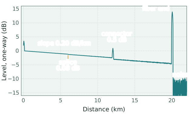
Simulated trace of 20 km of fiber at 1550 nm with a 1 µs pulse (102 m at ), 0.20 dB/km attenuation and a backscatter coefficient of −51 dB for that pulse, plotted as one-way loss ( of the returned power) as OTDRs display it. Events: a 0.08 dB fusion splice at 6 km, a 0.5 dB connector with −45 dB reflectance at 12 km, and a cleaved end at 20 km, taken as 4 % reflectance, the usual round figure (silica's index gives 3.4 %).
The simulated trace shows the features of a real one. At 0 km the reflection from the instrument's own connector produces a peak, and the first stretch of fiber is hidden in its dead zone. The backscatter then falls along a straight line whose slope, 0.20 dB/km, is the attenuation of the fiber; a change of slope marks a section of different fiber or of distributed loss. The splice at 6 km is a 0.08 dB step with no peak, since a good fusion splice has no index step to reflect from, and the connector at 12 km is a 0.5 dB step with a reflection peak. The cleaved end at 20 km gives the largest peak, 18.5 dB above the backscatter, followed by the noise floor of the receiver. The end of a fiber is placed at the start of its reflection; a break that does not reflect, such as a crushed one, shows only as the point where the backscatter drops into the noise.
| Feature | Trace appearance | Cause |
|---|---|---|
| Continuous slope | Exponential decay (in log power vs distance, a straight line) | Fiber Rayleigh attenuation |
| Step down | Sudden drop without reflection peak | Lossy splice or bend |
| Step down + peak | Drop with reflection peak | Connector (lossy + reflective) |
| Step up | Sudden increase | Splice between dissimilar fibers (backscatter coefficient mismatch) |
| Sharp peak then noise | Fresnel reflection at large step, then noise | Fiber end, break, or open connector |
| Saturation | Receiver overload | Strong reflection (e.g., return from end facet of un-terminated fiber) |
| Isolated peak, no step | Reflection with no loss across it, often beyond the fiber end | Ghost: echo of a strong reflection |
A peak with no loss step across it, often beyond the end of the fiber, is most likely a ghost: light from a strong reflection that has been reflected again, usually at a connector near the instrument, and has made a second round trip, so that it appears at a multiple of the real event's distance. Compared with the real reflection, the echo has been reflected twice more, once at the extra reflector and once more at the real one, and has made another round trip through the fiber, and each of these takes its share of the power. If the front connector in the figure reflected −45 dB, as the connector at 12 km does, the echo of the end reflection would appear at 40 km with 68 dB less power than the end reflection itself: 45 dB at the front connector, 14 dB at the end a second time and 9.2 dB for the extra round trip. An open front connector reflecting 4 % would raise it by 31 dB. A clean, low-reflectance connection at the instrument, such as an angled connector, is the remedy. Ghosts also appear when the range setting is shorter than the fiber, so that light from one pulse returns after the next is launched and is drawn at the wrong distance.
Two wavelengths separate bends from splices. The loss of a bend rises steeply with wavelength (macrobend loss) while that of a splice hardly changes, so a step that is larger at 1550 or 1625 nm than at 1310 nm marks a bend. A step up at a splice is a gainer, discussed below.
Distance, loss and reflectance scales
The position of any feature corresponds to time-of-flight: , where is the group velocity and the factor of 2 accounts for the round trip. Corning specifies at 1550 nm and 1.4676 at 1310 nm for standard single-mode fiber (speed of light in fiber); either gives 102 m per microsecond, as does the rounded 1.47 used for the figure. The distance scale is only as accurate as the index entered in the instrument: an error of 0.001 in moves a feature at 20 km by 14 m. The length measured is that of the fiber, which in a cable is generally longer than the cable because the fibers are laid in with some excess length.
Because the light makes a round trip, a loss of dB before a point lowers the power returned from it by dB. OTDRs therefore plot of the returned power, so that the slope reads directly as the one-way attenuation coefficient and a step as the one-way loss of an event. Reflectance, the negative of return loss, and the backscatter coefficient are quoted on the ordinary scale.
The backscatter coefficient is the power backscattered from the start of the fiber divided by the launched peak power. Light arriving at any instant comes from a length of fiber , half the length that a pulse of duration occupies in the fiber, so is proportional to : the figure's −51 dB at 1 µs becomes −71 dB at 10 ns. A reflection of reflectance adds times the incident power to the backscatter, so its peak stands above the backscatter by
which instruments invert to report reflectance, . The 18.5 dB end peak in the figure gives , the 4 % taken for the cleaved end. With a 10 ns pulse the same end would stand 28.5 dB high, because falls with pulse width and does not. Peak height alone therefore does not give reflectance, and a reported reflectance is only as accurate as the backscatter coefficient the instrument assumes.
Pulse width, resolution and dynamic range
The pulse width sets both the resolution and the reach. Events closer together than the length the pulse occupies on the trace merge into one, so the two-point resolution is about
the same length that sets the backscatter coefficient. At fixed peak power a longer pulse carries more energy and returns proportionally more backscatter. With receiver noise dominant and a fixed receiver bandwidth, the one-way dynamic range therefore rises by 5 dB per factor of ten in pulse width; if the bandwidth is narrowed in step with the pulse, the noise also falls as and the gain approaches 7.5 dB per decade. For and the figure's fiber:
| Pulse width | Resolution | Backscatter coefficient | Dynamic range relative to 1 µs |
|---|---|---|---|
| 10 ns | 1.0 m | −71 dB | −10 to −15 dB |
| 100 ns | 10.2 m | −61 dB | −5 to −7.5 dB |
| 1 µs | 102 m | −51 dB | 0 |
| 10 µs | 1.02 km | −41 dB | +5 to +7.5 dB |
| 20 µs | 2.04 km | −38 dB | +6.5 to +9.8 dB |
The first value in the last column is for a fixed bandwidth, the second for a bandwidth scaled with the pulse. Going from 10 ns to 1 µs gains 10 to 15 dB, the loss of 50 to 75 km of fiber at 0.20 dB/km, and coarsens the resolution a hundredfold, from 1.0 m to 102 m.
Averaging improves the signal-to-noise ratio more slowly: the noise falls as the square root of the number of averaged traces , which adds dB to the one-way dynamic range, so ten times the averaging time gains 2.5 dB. Only one pulse may be in the fiber at a time, which for 20 km of fiber, a 196 µs round trip, limits the pulse rate to 5.1 kHz. The usual choice is the shortest pulse that still gives a clean trace at the far end: long pulses for long spans, short ones for closely spaced events such as the connectors in a building, often both in turn on the same fiber.
Dynamic range and how it is specified
Dynamic range is the difference, on the one-way scale, between the backscatter level at the start of the fiber, extrapolated back along the straight part of the trace, and the noise level of the receiver. It is quoted for the longest pulse, at each wavelength, after a stated averaging time, and datasheets commonly take the noise level as the RMS noise (SNR = 1). Definitions based on a higher noise level give a smaller number for the same instrument, so values compare only under the same definition, pulse width and averaging time. As a one-way figure it compares directly with fiber loss: at 0.20 dB/km, 10 dB is 50 km.
Small events can be measured over only part of that range. For the noise on the trace to fall to 0.1 dB, the detected backscatter must be 21.2 times the RMS noise, since dB; that is dB above the SNR = 1 level. Loss measurements fit the trace over a stretch on each side of an event, which averages some of the noise away, but splices of a few hundredths of a dB are still measured well inside the dynamic range. A strong reflection can be located much closer to the noise: the fiber end in the figure stands 18.5 dB above the backscatter.
Dead zones
After a strong reflection the trace is unusable for some distance: the reflected pulse occupies its own length of the trace, and the overdriven receiver needs time to recover. Two specifications describe this.
- The event dead zone is the minimum distance after a reflective event at which a second reflective event appears as a separate peak and can be located. It is set by the pulse length and the receiver bandwidth, and it cannot be shorter than the two-point resolution: 1.0 m at 10 ns, even for an ideal rectangular pulse and a receiver fast enough to follow it.
- The attenuation dead zone is the minimum distance after a reflective event at which the loss of a following event can be measured, which requires the trace to have settled back onto the undisturbed backscatter. It is the longer of the two, and it grows with the reflectance of the first event, which sets how far the receiver is overdriven.
Datasheets give both for the shortest pulse and a stated reflectance; at the longer pulses used on long fibers they are correspondingly longer. The event dead zone decides whether two connectors a few meters apart in a patch panel appear as two events, the attenuation dead zone whether a splice just after a connector can be measured.
The first dead zone on every trace is at the instrument's own connector. A launch fiber (launch cable) between the OTDR and the fiber under test moves the link's first connector out of it, so that the connector has backscatter on both sides and its loss and reflectance can be measured; a receive fiber at the far end does the same for the last connector. Each must be longer than the attenuation dead zone at the pulse width in use, so at least : 102 m at 1 µs, 2.0 km at 20 µs.
Gainers and bidirectional measurement
The backscatter level on each side of a splice depends on the fibers as well as on the loss between them. A fiber's backscatter coefficient is set by its Rayleigh scattering coefficient and by the fraction of the scattered light that its guided mode recaptures, which in single-mode fiber scales approximately as , with MFD the mode field diameter. If the second fiber backscatters more strongly than the first, the trace drops by less than the splice loss, or rises: a gainer. Measured from the other end, the same splice shows too much loss. With the true loss and the difference in backscatter coefficient in dB, the losses read from the fiber-1 end and from the fiber-2 end are
where the factor of one half puts on the one-way scale. Their mean is .
Take the splice from a fiber of 10.4 µm mode field diameter to one of 9.2 µm used in the fusion splicing entry. The mode mismatch costs dB, and counting only the difference in recapture, the smaller-mode fiber returns dB more backscatter, so that dB. Read from the 10.4 µm side, the splice gives dB, a gain; from the other side, dB. Real fiber pairs also differ in Rayleigh coefficient, which changes the size of the error but not the correction, since the average of the two directions cancels any difference in backscatter coefficient. Splice acceptance, particularly where different fiber types meet, is therefore based on bidirectional measurements averaged event by event.
Reading fiber attenuation from the trace slope, and why splice losses need bidirectional averaging, is covered in How to Measure Fiber Attenuation and Bend Loss.
Coherent, phase-sensitive and inelastic OTDR
A conventional OTDR detects the returned power directly, using a laser whose spectrum is broad enough that interference between light scattered from different points averages out. Coherent OTDR uses a narrow-linewidth laser and mixes the backscatter with a local oscillator split from the same laser; a frequency offset between probe and oscillator puts the beat at an intermediate frequency, where it is detected in a narrow electrical bandwidth (heterodyne detection). The local oscillator raises the weak backscatter above the receiver noise, and the narrow bandwidth rejects most of the amplified spontaneous emission of in-line amplifiers, which is why coherent OTDR is used on long-haul and submarine links. The isolators in each amplifier block backward-traveling light, so submarine repeaters include a loopback path that couples backscatter from the outgoing fiber into the return fiber of the pair, and the backscatter from each span reaches the terminal through the amplifiers of the opposite direction. With a coherent source the backscatter is a random interference pattern whose level fades in and out along the fiber, and instruments average over several optical frequencies to smooth the trace.
The name coherent OTDR is also used for phase-sensitive OTDR (φ-OTDR), which follows the phase of the coherent backscatter from pulse to pulse and so records strain along the fiber as it changes in time. It is the basis of distributed acoustic sensing.
Inelastic scattering gives two sensing variants. Brillouin OTDR (BOTDR) measures the frequency shift of the Brillouin backscatter, which depends on strain and temperature; Raman OTDR (ROTDR), usually called distributed temperature sensing (DTS), uses the ratio of anti-Stokes to Stokes Raman backscatter, which depends on temperature. Both locate each measurement by time of flight.
For short paths, optical frequency-domain reflectometry (OFDR) sweeps a laser's frequency instead of timing a pulse and resolves features less than a millimeter apart over tens of meters, the scale of components and photonic circuits, where an OTDR resolves meters over kilometers.
Typical instrument parameters
| Parameter | Typical range |
|---|---|
| Pulse width | 5 ns – 20 μs |
| Spatial resolution | 0.5 m – 2 km (set by pulse width: ) |
| Dynamic range | 25 – 50 dB |
| Operating wavelength | 1310, 1550, 1625 nm (matching telecom bands) |
| Dead zone | 0.5 – 30 m (region near launch where strong launch reflections mask features) |
Applications and limitations
- Installation verification: confirms each splice meets specification ( 0.1 dB loss)
- Fault location: locates a break to within the resolution of the pulse and the accuracy of the group-index setting
- Loss budget verification: confirms link total loss matches design; the end-to-end loss measured with a light source and optical power meter remains the reference (see Measuring Insertion Loss and Return Loss)
- Long-term monitoring: detects gradual degradation (bends, water ingress)
- Splice acceptance testing: bidirectional OTDR measurement averages splice loss measurements from both directions
The method depends on backscatter. An air core produces almost no Rayleigh backscatter, so hollow-core fiber gives a faint trace, and in amplified links the backscatter stops at the isolator of the first amplifier, the case that coherent OTDR addresses.
Common questions
What does an OTDR measure?
The power returning from a fiber against time after each pulse: Rayleigh backscatter from the glass and reflections from connectors, breaks and the far end. Time converts to distance at 102 m per microsecond and the backscatter level to loss, so one trace gives the attenuation of the fiber and the position, loss and reflectance of each event.
How is OTDR dynamic range specified?
As the one-way difference between the backscatter level extrapolated to the start of the fiber and the noise level, for the longest pulse after a stated averaging time, commonly at SNR = 1. Measuring small events needs more: 0.1 dB of noise on the trace requires the backscatter to be 6.6 dB above the SNR = 1 level.
What is the difference between the event dead zone and the attenuation dead zone?
The event dead zone is the shortest distance after a reflection at which a second reflection shows as a separate peak; the attenuation dead zone, which is longer, is the shortest distance at which the loss of a following event can be measured. Both grow with pulse width and with the reflectance of the first event.
Why does an OTDR show a gain at some splices?
Because the fiber after the splice backscatters more strongly than the one before it, often because its mode field diameter is smaller. From the other end the same splice shows too much loss, and the mean of the two directions is the true loss.
What is coherent OTDR?
An OTDR that mixes the backscatter with a local oscillator from the same narrow-linewidth laser. Its narrow detection bandwidth rejects amplifier noise, so it can test long-haul and submarine links through their amplifiers; the phase-sensitive form, φ-OTDR, is the basis of distributed acoustic sensing.
References: M. K. Barnoski and S. M. Jensen, "Fiber waveguides: a novel technique for investigating attenuation characteristics," Applied Optics 15, 2112 (1976). E. Brinkmeyer, "Analysis of the backscattering method for single-mode optical fibers," Journal of the Optical Society of America 70, 1010 (1980). P. Healey, "Fading in heterodyne OTDR," Electronics Letters 20, 30 (1984). D. Derickson (ed.), Fiber Optic Test and Measurement (Prentice Hall, 1998). A. H. Hartog, An Introduction to Distributed Optical Fibre Sensors (CRC Press, 2017). Telcordia GR-196-CORE, Generic Requirements for Optical Time Domain Reflectometer (OTDR) Type Equipment. IEC 61746-1, Calibration of optical time-domain reflectometers (OTDR), Part 1: OTDR for single mode fibres. Corning, SMF-28 Ultra Optical Fiber product information (effective group index).