Glossary entry

Knife-edge measurement

A beam-profiling technique that measures transverse beam intensity profile by translating a sharp opaque edge across the beam and recording the transmitted power. The standard simple beam-width measurement.

Optics & beams Lab practiceUpdated October 2026

The knife-edge technique measures the transverse profile of a focused or collimated laser beam by translating a sharp opaque blade across the beam path and recording the power passing the blade as a function of blade position.

Geometry.

The transmitted power $P (x)$ as the blade moves across the beam at position $x$ is the complementary error function for a Gaussian beam:

P (x) = \frac{P_{0}}{2} erfc ⁣ (\frac{\sqrt{2} (x - x_{0})}{w}),

where $P_{0}$ is the total beam power, $x_{0}$ is the beam center, and $w$ is the $1 / e^{2}$ beam radius. The function transitions from $P_{0}$ (blade fully out) to 0 (blade fully blocking) over a characteristic width set by $w$ .

Width extraction. The 10–90 % transition width $Δ x_{10 / 90}$ is most commonly used:

Δ x_{10 / 90} = x_{10 %} - x_{90 %} \approx 1.28 w,

where $x_{P %}$ is the blade position at which the transmitted power is $P %$ of the unblocked value. The 1.28 factor is for an ideal Gaussian; real beams may deviate by a few percent.

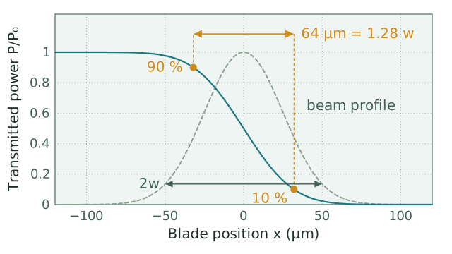
Knife-edge scan: transmitted power against blade position, an error-function curve whose 10 to 90 percent width is 1.28 w. — Computed $P (x) / P_{0} = \frac{1}{2} e r f c (\sqrt{2} x / w)$ for a Gaussian beam with $w = 50$ µm and $x_{0} = 0$ , with the beam's intensity profile dashed. The 90 % and 10 % points fall at $\mp 32.0$ µm, 64.1 µm apart, which is $1.28 w$ ; the $1 / e^{2}$ radius is where the dashed profile falls to 13.5 % of its peak.

Other commonly used measures:

Measure	Relation to $w$	Notes
15.9–84.1 % width	$1.00 w$	Equals $2 σ$ (1-sigma full width)
10–90 % width	$1.28 w$	Most common; standard convention
5–95 % width	$1.64 w$	Uses more of the tails; more sensitive to background offset and detector noise

Practical setup. A typical knife-edge measurement uses a razor blade or polished metal edge mounted on a motorized linear translation stage with sub-micron resolution. A large-area photodetector (much larger than the beam) is placed immediately behind the blade, removing any sensitivity to beam steering or detector position. The blade is stepped across the beam in $\sim$ 100 to 1000 steps, recording transmitted power at each position.

Advantages. Robust to beam imperfections (insensitive to non-Gaussian shape in the orthogonal direction). Single-axis at a time, but two orthogonal scans (X and Y blade orientations) suffice for separable beams. Requires no specialized hardware beyond a translation stage and a photodetector. Works for beams from UV to far-IR (limit set by detector and blade material).

Limitations. Single-axis at a time. Does not capture full 2D profile. Assumes the beam is separable (Gaussian or near-Gaussian) in both axes. For non-Gaussian or strongly astigmatic beams, the orthogonal-axis profile is implicitly averaged and useful information is lost. Multi-mode beams produce non-erfc transitions and require numerical fitting rather than simple width extraction.

Comparison to other techniques.

Technique	1D vs 2D	Resolution	Sensitive to non-Gaussian?
Knife-edge	1D, repeat for orthogonal	sub-μm	No (averages orthogonal axis)
Slit scan	1D, repeat for orthogonal	sub-μm	No (better tolerance than knife-edge for asymmetric beams)
Pinhole scan	2D (raster)	depends on pinhole	Yes; captures full 2D profile
Camera/CCD	2D direct	pixel-limited	Yes
$M^{2}$ measurement	Multi-Z 1D	combines knife-edge or camera	Yes; quantifies non-Gaussian content

ISO 11146 specifies the second-moment width ( $D 4 σ$ ) as the formal beam diameter for all beam-quality characterization. For an ideal Gaussian, the 10–90 % width divided by 1.28 gives $w$ , and $2 w$ equals $D 4 σ$ ; for real beams the two diameters can differ by 5–20 %. For research and qualification, $M^{2}$ measurement (which combines knife-edge or camera widths at multiple Z positions) is the standard; for quick bench measurement, knife-edge alone is sufficient and is the workhorse of laser laboratories.

Knife-edge widths measured at several distances feed the M² measurement procedure.